EIF-Services

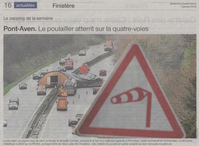
Here is an application of Basilisk based on a funny news item: a large henhouse took off on January 1^st 2018 during the Carmen storm, which blew at more than 100 km/h in Brittany (inland). The henhouse (and the chicken!) landed on a four-lane highway:

The exercise reported here consists in computing the lift force exerted by the wind on the structure (before take-off) in order to better size its fastening to the ground, for example.

A Blender model of the henhouse was first set up (by eye as far as this portfolio is concerned¹):

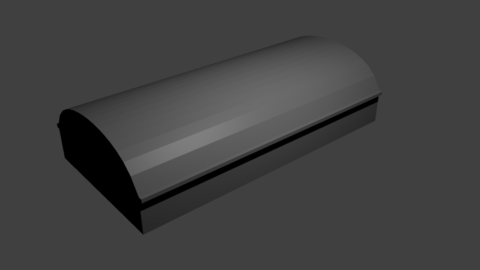
The dimensions of this model are 4 m x 8,4 m x 16 m. The height of the (prototype) henhouse (4 m) will be referred to as L. The "blend" was then exported to STL format so that Basilisk can read it:

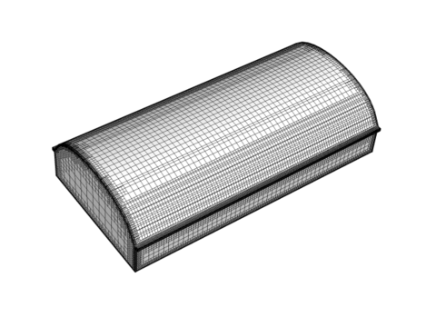
N.B. The figure above already exhibits the adaptive nature of the mesh generated by Basilisk: resolution increases only where it is necessary.

The following animation provides a first insight into the 2D simulation of a 108 km/h wind (the speed of which will be known as U from now on):

This was about vorticity. The video is deliberately compressed, but the structure of the pressure and velocity fields is detailed below:

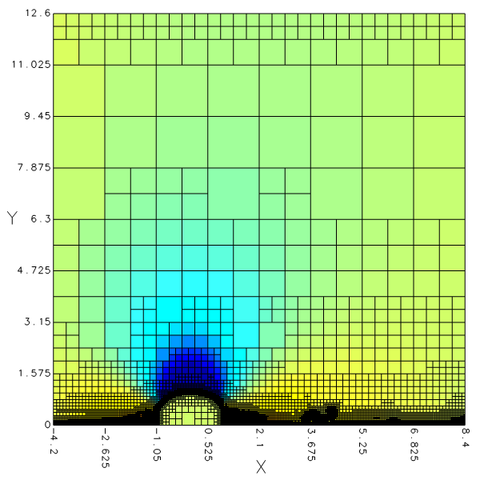
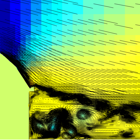
N.B. The auto-adaptivity of the mesh is clearly demonstrated by the last visualization.

The main result, however, is contained in the next figure, showing the temporal evolution of the lift (y) and drag (x) forces² due to either pressure (P) or friction (F):

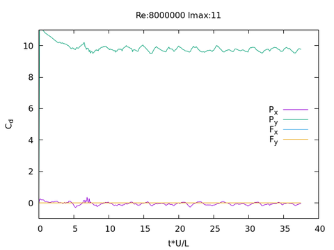
The simulation evolves to a stationary state (but not a permanent one, as already seen in the video). Furthermore the P_y coefficient is clearly much stronger than the other ones; let us recall that P_y is the lift force due to the pressure field surrounding the henhouse. Friction forces are negligible, at least when U = 108 km/h: they cannot even be seen on the graph (but will be on the next one). During the stationary regime P_y oscillates around 9.74 (value obtained when averaging after nondimensional time t*U/L = 25), meaning a vertical force² equal to 9,74*0,5*1,2*30²*4 ~ 34300 N for each meter in the crosswind direction! Such a force is equivalent to the weight of 3.5 tons: hence a 108 km/h wind definitely appears to be able and lift off a structure such as our henhouse...

These results are robust, aren't they?

As with any numerical modelling, the question arises whether the resolution used is sufficient. The Reynolds number for the flow under consideration is Re = U*L/ν_air = 30*4/(1,5·10^-5) = 8·10⁶. DNS cannot deal with such a value, unless using a supercomputer. Thus one has to get into some sort of turbulence modelling such as LES (or RANS when conditions are met), which was not done for this demo. However there are solutions in the Basilisk community and turbulence modelling is the subject of an active technological watch by EIF-Services.

Nevertheless the goal here was only to compute an aerodynamic lift, which appeared to be mainly due to the pressure field; and such a lift has converged at the resolution used here (lmax = 11), as shown in the following graph:

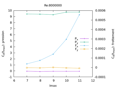
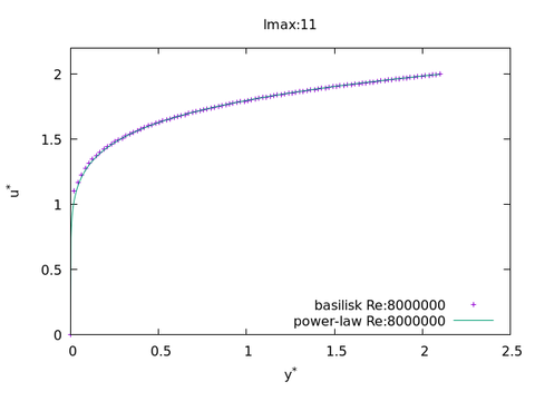
Basilisk resolution is defined by lmax, the maximum depth allowed to the tree structure of the self-adaptive mesh (the maximum resolution is multiplied by 2 when lmax is increased by 1). The figure above shows that F_x alone still depends in the resolution at lmax = 11 but as already noticed F_x and F_y are very small compared to P_x et P_y (the scale for the latter is on the left of the plot). This is consistent with boundary layer theory (in the absence of flow separation), according to which wall pressure is determined par the large scales of the flow. Flow separation itself depends on the details of the boundary layer but the latter appears to be well reproduced at lmax = 11, as demonstrated by this last plot comparing the Basilisk velocity on flat wall (henhouse removed) to the Prandtl power law³ (imposed anyway at the upstream boundary):

All these arguments support the robustness of the results obtained so far, at least if one focuses on the forces experienced by the henhouse. The realism of study would then profit by a 3D modelling⁴ and/or taking into account surface roughness. According to us however, numerical modelling aims at providing reliable orders of magnitude based on a reasonably simplified prototype, while not claiming to replicate every detail of the real thing. Anyway the implementation of numerical models and the interpretation of their results requires scientific expertise, such as provided by EIF-services.

1. ↑Of course a real study would be based on in situ measurements, or a 3D model provided by the Client.
2. ↑Here the lift or drag forces are drawn in the form of nondimensional coefficients defined by the ratio of the corresponding force by the product 0,5*ρ_air*U²*L, where ρ_air = 1,2 kg/m³ (air density), U = 108 km/h = 30 m/s (wind speed) et L = 4 m (height of the henhouse). The "force" referred to here is actually the force per unit length in the crosswind direction (2D simulation).
3. ↑Franck M. White (2016): Fluid mechanics p.420-421 (eq7.39-7.42).
4. ↑A first approach is given by the visualization below, obtained at the end of a simulation with lmax = 7. This is the pressure field; the structure and amplitude in the middle of the barn are quite comparable to those obtained in 2D (except that the color scale is different here).